A friendly tour · v0.7
Spiking neural
networks are
convex optimizers.
A population of leaky integrate-and-fire neurons, with the right connectivity, solves a constrained convex program. Between spikes the state drifts down the gradient. When it crosses a constraint, a spike resets it onto the wall. The constraints that keep firing are the ones active at the optimum. Below is a real solve; drag to look around.
- Install
pip install snn-opt- Constraints
- Linear · conic
- Backends
- Python · C++
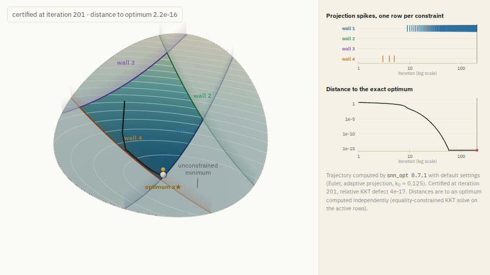
The bowl is the objective of a 2-D quadratic program; the coloured
walls are its four linear constraints. Watch the network
search: wall 4 fires for three steps and falls silent, then
wall 1 is recruited and fires on every step until the optimum. The
marker has no momentum: the dynamics are a first-order flow, drawn on
the surface for intuition. Every position and every spike is output
from snn_opt.
Three beats
The idea, distilled.
The whole framework collapses into three repeating moves. Everything else, the convergence proofs, the hardware story, the spike raster, falls out of these.
Drift.
Between spikes, each neuron's membrane voltage moves by the gradient of an objective. Plain gradient descent, dressed up as biology.
Spike.
When the voltage would push the trajectory past a constraint, a spike fires. The spike re-projects the state onto the feasible boundary: a discrete correction.
Settle.
At the optimum the drift into the active walls is exactly balanced by their spikes. Which constraints keep firing is the active set, and their firing plays the role of the KKT multipliers.
A picture
What it
looks like.
An 8-D quadratic whose optimum lies outside a 16-facet polytope. Each dot is one projection event. Watch the network search: one facet fires a short burst and falls silent, three more are recruited in turn and then fire on every step. Those three are exactly the constraints active at the true optimum.
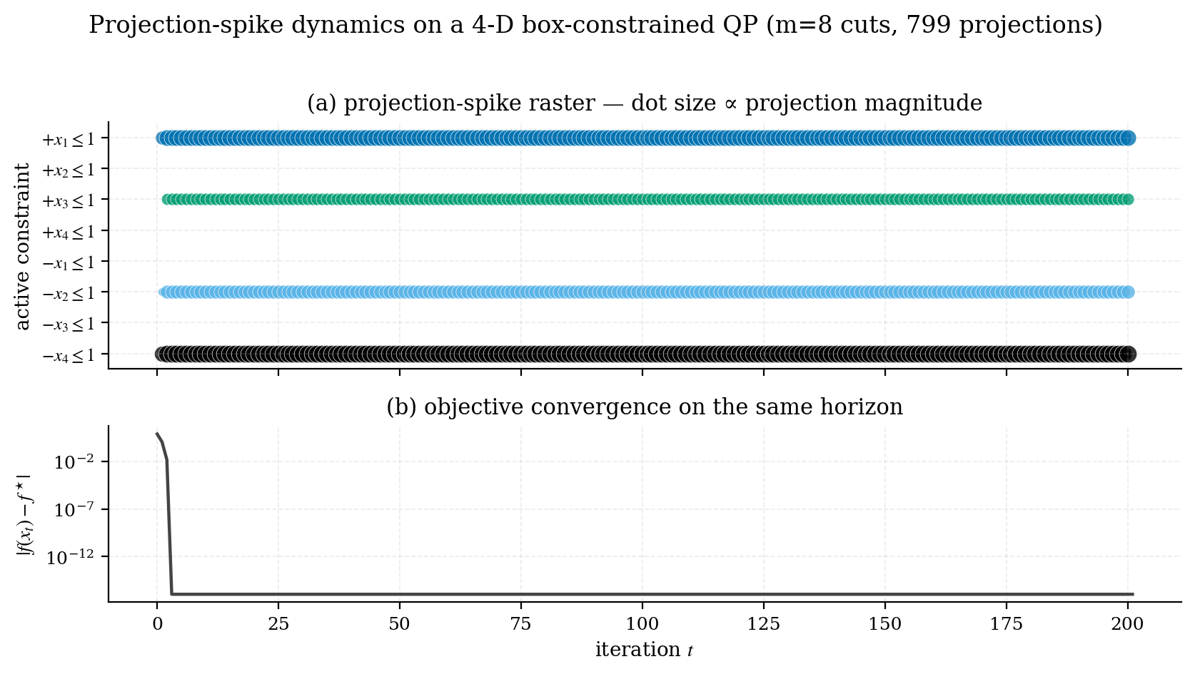
benchmarks/02_spike_raster.py.
Beyond polytopes · new in v0.7
Curved walls
spike too.
Nothing in the drift-and-spike picture needs flat walls. Any convex set with a cheap projection joins the same spike sweep: balls, second-order and friction cones, the PSD cone, spectral-norm balls, and their intersections. Here a desired contact force would slip, so the network slides it around its friction cone to the nearest force that holds.
Certification
When to
trust the flag.
Since v0.6.0, converged=True is a
scale-invariant KKT certificate: a nonnegative
least-squares fit of the gradient onto the cone of facet normals,
with a complementarity guard, accepted only relative to the
problem's own gradient scale. The same problem certifies
identically at natural scale and at 1010×.

converged=False:
the certificate measures the cycle's relative KKT defect at 8.9e-4, above the default tolerance of 1e-4.
Generated by benchmarks/01_convergence.py.
The pre-0.6 test compared an absolute projected-gradient norm
against 1e-6, which had two structural defects: rescaling the
objective rescales every gradient, so on large-scale problems the
flag could never fire at any solution quality; and the old heuristic
removed each active facet's gradient component independently, so it
stalled at a cross-term residue whenever active normals were
correlated, even at the exact optimum. The new certificate fixes
both, and it cuts the other way too: it measures the
accuracy floor of the dynamics rather than flattering it, which is
why the benchmark above declines to certify at the default step size.
Results from v0.5 remain reproducible with
optimality_test="legacy_projected_gradient".
Accuracy
Where it
stops.
The dynamics converge to a fixed point of the discretised flow, which is not quite the minimiser of the QP. The offset shrinks with the gradient step, but a smaller step needs more iterations to arrive, so every iteration budget has its own best setting.
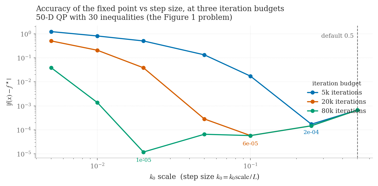
benchmarks/04_accuracy_tuning.py.
Three fields on the result expose different parts of the answer, and
they are worth checking on any real problem. joint_feasible reports
feasibility of the constraint rows, the bounds and any conic
constraints together.
kkt_residual is the KKT certificate value at the final
point (the section above), and exactly what converged now
certifies; the ratio kkt_residual / kkt_scale is the
normalized defect, comparable across problems and objective scalings.
projection_budget_exhausted flags a solve that ran out of
inner projection steps, which now aborts rather than being reported as
success. The repository README
has the full treatment.
Where does the offset come from? The projected-gradient fixed point
is the exact optimum whenever the projection is exact. The greedy row
sweep is exact when one wall is active (the solve at the top of this
page ends 2e-16 from the optimum), but not at a vertex where several
are. Since v0.7 you can hand the rows over as one exact joint
projector, joint_projector(C, d). On the 50-D problem
above, the objective gap then falls from the 6.7e-4 floor to 2.1e-10
under the default certificate, at the price of an inner Dykstra loop
per step.
Warm starts
Solve it again,
faster.
Receding-horizon control solves a nearly identical QP every tick, and the previous solution is an excellent first guess. On a sequence of 30 drifting QPs (checking convergence every 10 iterations), warm starting cuts a 221-iteration cold solve to 101 iterations, an essentially free 2.19×, with wall time falling in step (2.03×).

benchmarks/03_warm_start.py.
Map
What you'll
find here.
Six entry points. Pick whichever matches your appetite: the intuition essay, the conic extension, hands-on tutorials, the published papers, the source code, or the player itself.
- Intro essay · 8 min
The spiking idea explained from scratch, with no prior neuromorphic background required.
- Beyond polytopes new in v0.7
Cones, balls, PSD and spectral-norm constraints in the same spike sweep, with an interactive friction-cone solve.
- Tutorials hands-on
Walkthroughs: a five-minute quickstart, an SVM written as a QP, reading the spike raster, and grasp forces in friction cones.
- Papers peer-reviewed
The published work that uses this framework, with abstracts and DOI links.
- snn_opt repo source · Apache-2.0
Canonical Python implementation: solver, compiled C++ backend, a qualified KV260 FPGA reference, examples, benchmarks, full mathematical writeup.
- Full-screen player interactive
The solve from the top of this page in a full window: orbit, scrub through the steps, read the raster.
Install
Two lines
and you're in.
Prebuilt wheels for Linux (x86_64, aarch64), macOS (Apple Silicon), and Windows across CPython 3.9–3.14. The compiled C++ backend ships inside the wheel; no toolchain needed on your side.
pip install snn-opt
Then head to the Quickstart for a
five-minute walkthrough. The PyPI distribution name is
snn-opt (hyphenated, per PEP 503); the Python import
name is snn_opt. Pick the C++ kernel with
backend='c' for a roughly 10× speedup on the inner
projection loop. The same kernel source is HLS-compatible, and the
repository ships a physically qualified Kria KV260 reference
implementation under fpga/.
For whom
Who this is for.
Students starting a thesis on neuromorphic methods. Researchers from optimization or control who heard "spiking networks" and weren't sure what to make of it. Anyone who finds beauty in connections between fields that look unrelated until they don't.
If you want the formal version: head to the
snn_opt repository
for the full theory document, an academic-style README, and
a benchmark suite. The pages here are the
friendly version of the same material.
Acknowledgments
Acknowledgments.
Developed at the School of Artificial Intelligence, Taizhou University.
This codebase implements the SNN-QP research program led by Prof. Shuai Li (IEEE Fellow; Faculty of Information Technology and Electrical Engineering, University of Oulu, Finland), whose work on neurodynamic optimization originated this line of inquiry. The mathematical framework follows Mancoo, Keemink and Machens (NeurIPS 2020) and the broader projection-neural-network lineage (Hopfield–Tank, Kennedy–Chua, Xia–Wang, Liu–Wang).