A toy that explains the whole thing
Imagine a single point living in a flat 2-D plane. Two things act on it:
-
A pull. There’s a target somewhere, and our point feels a force pulling it toward at every moment. That force is the gradient of an objective, say , and the point moves in the direction that decreases .
-
A wall. There’s a line (or two) that the point can’t cross. Each wall is an inequality constraint: .
If there were no walls, the point would just glide to , which is plain gradient descent. The interesting question is what happens when the gradient pulls the point into a wall.
The spike
Here’s the move. Between collisions, the point drifts by a small step in the gradient direction. Just before it would cross a wall, a spike fires: a discrete correction that pushes the point back to the wall, exactly along the wall’s normal, by exactly the amount needed to stay on the feasible side.
That’s it. That’s the whole algorithm: drift, spike, drift, spike. The drifts shrink the objective; the spikes preserve feasibility. Eventually the two balance, and the point sits at the constrained optimum.
The picture below shows what this looks like on an 8-D problem with sixteen walls. Each row is one wall and each marker is one spike at that wall, sized by how big the spike was. Only four walls ever fire, and only three of those keep firing: those three are the walls the solution actually rests against.
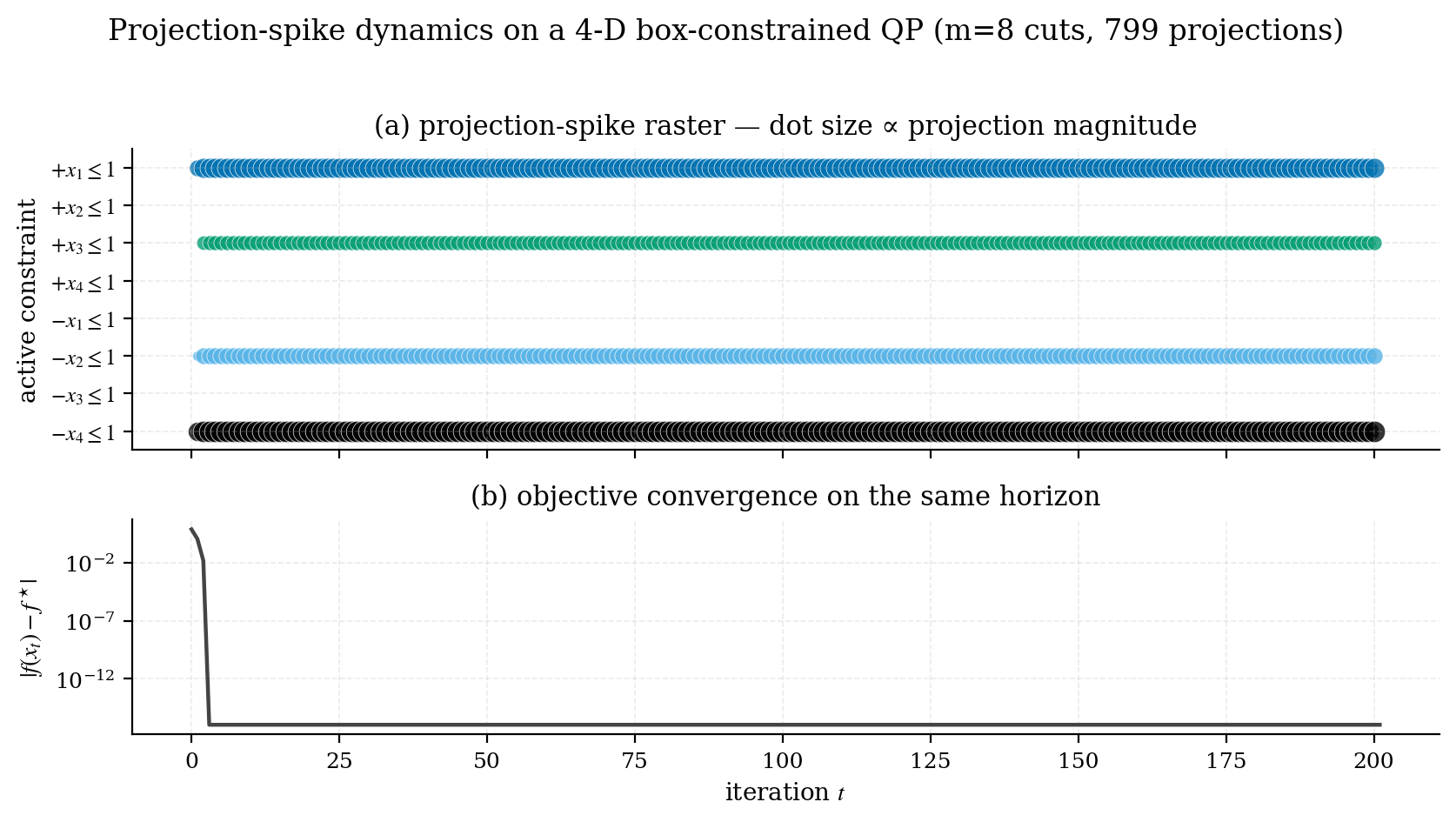
benchmarks/02_spike_raster.py in the snn_opt repository.Why call it spiking?
A leaky integrate-and-fire (LIF) neuron has a very simple dynamic: its voltage drifts according to its inputs, and when crosses a threshold , it fires a spike and resets. Repeat.
If you write down those dynamics for a population of LIF neurons with the right recurrent connectivity, you get exactly the system above:
where is a sum of delta functions, the spike train. The threshold-crossings of the LIF model and the constraint-violations of the optimizer are the same event, viewed from two angles. Each spike is a primal-dual update.
This isn’t a metaphor. It’s a literal equivalence first formalized by Mancoo, Boerlin and Machens at NeurIPS 2020, and the snn_opt library is a clean Python implementation of the discretized version.
What does this buy us?
Three useful things:
- A new way to think about classical solvers. Many things you already know (projected gradient methods, primal-dual algorithms, active-set methods) fall out as discretizations of this single dynamic. The spike raster is a diagnostic that doesn’t exist in their classical form.
- Hardware naturalness. The primitives are matrix-vector multiplies, comparisons, and resets. Those are exactly the operations digital neuromorphic chips are good at (Loihi, SpiNNaker, TrueNorth).
- A unifying lens for ML. A surprising number of classical machine-learning problems can be cast as constrained QPs and solved by exactly the same dynamics. Portfolio optimization is the worked example in the published paper; a broader series of such reductions is in progress.
Where to go next
- Quickstart: install
snn_opt, solve your first QP in five lines of Python. - SVM as a QP: turn a textbook SVM dual into something the solver can run, end to end.
- Reading the spike raster: what the dots mean, what they tell you about your problem, and what to look for when something is wrong.
If you want the math in full, including the eigenvalue-based step-size choice and the convergence analysis, head to docs/theory.md in the repo. The main README has the academic-paper presentation; this site is the friendly version of the same material.